The Breker Trekker Tom Anderson, VP of Marketing
Tom Anderson is vice president of Marketing for Breker Verification Systems. He previously served as Product Management Group Director for Advanced Verification Solutions at Cadence, Technical Marketing Director in the Verification Group at Synopsys and Vice President of Applications Engineering at … More » Mystic Secrets of the Graph – Part TwoDecember 3rd, 2015 by Tom Anderson, VP of Marketing
Last week, we began exploring some of the ancient, mysterious powers of graph-based scenario models to show their power for verification and ability to capture the verification space, many aspects of the verification plan, and critical coverage metrics. We’re just kidding about the first part; there’s nothing at all mystical or magical about graphs. In fact, this series of posts is intended to show the opposite and demonstrate with a easy-to-follow example the value of graphs. As we noted in our last post, graph-based scenario models are simple in concept: they begin with the end in mind and show all possible paths to create each possible outcome for the design. They look much like a reversed data-flow diagram, with outcomes on the left and inputs on the right. An automated tool such as Breker’s Trek family can traverse the graph from left to right, randomizing selections to generate test cases that can run in any target platform.
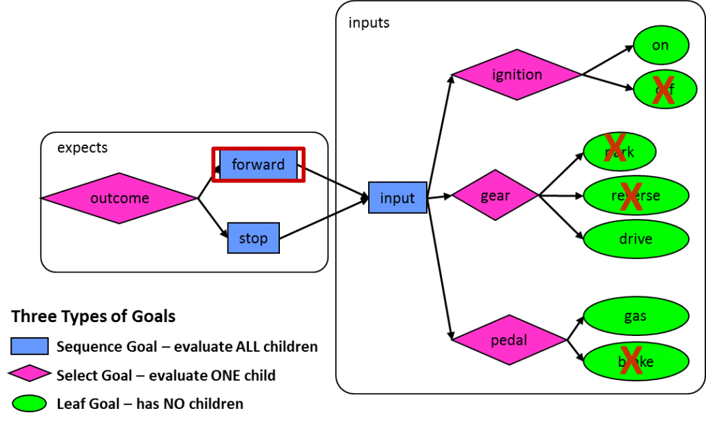
The example we introduced was a graph-based scenario model that shows how to verify that a car can move forward or stop. We showed a fully elaborated model where the inputs (ignition, gear, and pedals) were set appropriately for each of these two scenarios. However, such a non-convergent graph (essentially a tree) expands very quickly for any real IP or SoC design. You need to have convergent graphs that can share rather then replicate portions used for multiple scenarios. The solution is graph constraints, which control how the graph will be traversed when generating test cases. For example, the following graph shows constraints that set the inputs the proper way to produce the result of the car moving forward: You can read the constraints in this graph as “if the outcome is to move the card forward, the ignition must be on, the gear must be in drive, and the gas pedal must be pushed.” The outcome of stopping the car can be shown on the same graph with an additional set of constraints, specifying that the ignition must be on, the gear must be in reverse or drive, and the brake pedal must be pushed: Constraints limit traversal of the graph to paths that are legal according to the specification of the design. There are other uses of constraints, for example to focus the generated test cases on a particular portion of the functionality. If this graph was being used to test a car whose reverse gear was broken, the graph could be constrained so that the reverse option would never be selected for the gear. This situation is quite common in SoC verification when some of the RTL has not yet been implemented and so it makes no sense to generate test cases yet for that part of the design. Biasing selections so that all options are not considered equally can be considered another form of constraint. In a graph-based scenario model, adding a number to a selection biases graph traversals. For example, the following annotation to the gear selection specifies that for every ten walks through the graph, on average six will choose the gear to be in park, three will choose drive, and one (default value) will select reverse:
Our final post in the series will show how to expand this graph by adding system-level scenarios and how to repeat portions of the graph in a single traversal. We will also discuss system-level coverage metrics in the context of this particular example. Until then, please comment on whether this series is useful for you and please let us know if you have any questions. Tom A. The truth is out there … sometimes it’s in a blog. Tags: Accellera, Breker, constraints, EDA, functional verification, goal, graph, graph-based, horizontal reuse, node, portable stimulus, PSWG, randomization, scenario model, scheduling, simulation, SoC verification, test generator, Universal Verification Methodology, uvm, vertical reuse, VIP Warning: Undefined variable $user_ID in /www/www10/htdocs/blogs/wp-content/themes/ibs_default/comments.php on line 83 You must be logged in to post a comment. |
|
|
|||||
|
|
|||||
|
|||||


